How we reduced the latency of a CDN by 40%

You're about to Netflix and Chill, you finally agree on something to watch and you click play, how does that video stream come back so fast? You wouldn't want your network to get performance anxiety when the time comes to deliver. There is a lot of impressive engineering that goes into making sure that does not happen.

In 2023 I was working at Protocol Labs on distributed systems, and I was part of a team building a decentralized CDN network called Saturn. At its peak, Saturn served 2 billion requests to around 80 million clients each week. It took Saturn 1 year to reach 4,000 nodes, becoming the fastest growing and largest CDN network in history by PoP size with a capacity of 150Tbps (half of Cloudflare's at the time). To bring Saturn to a competitive level in the CDN world required a ton of optimization. In the world of networking, optimization is unintuitive. The path between two points is almost never a straight line. The fastest path is not necessarily the shortest one. Optimizing blindly for one metric can cause another metric to tank completely. The list goes on...

Optimizing Saturn was a huge engineering undertaking. For this post, I'll give a glimpse into our work into optimizing one of the most important numbers for any CDN: latency.

The Problem

Content Delivery Networks (CDNs) are systems of distributed servers that deliver content to users based on their geographic location. Some of the primary use cases for CDNs is to offer speed, reliability, and scale for distributing content around the web. So instead of having to worry about upgrading and scaling your servers when your app blows up, you pay a CDN like Saturn to do that work for you.

Saturn was not a typical CDN, it was decentralized. In this setting, we allowed people from around the globe to contribute with their own hardware to become a node on the network that caches and serves files. Those people got paid depending on their contribution to the CDN. We did have minimum hardware requirements of course, notably a minimum of 10Gbps uplink. We hypothesized that decentralizing the network would give us the following benefits:

• Resiliency: the network was extremely robust against outages.
• Proximity: we can have nodes closer to users than any other centralized CDN network.
• Scale: the network organically scales with demand and it can scale faster than any CDN.

Whether decentralization was the right call or not is a topic for another post. For now, we'll just assume that is a constraint that we have to deal with, and one that does have considerably challenging consequences. The core problem we will focus on in this post is selecting the optimal nodes to serve content to each client. This problem is significantly more complex than in traditional, centralized CDNs due to several factors:

• Heterogeneous Node Characteristics: Nodes in the network have diverse hardware specifications, and network connections. This variability makes it difficult to predict and rely on consistent performance across the network.
• Dynamic Network Conditions: Network latency, bandwidth, and reliability can fluctuate rapidly due to factors beyond our control, such as internet service provider issues or local network congestion.
• Scale and Distribution: With millions of clients and thousands of nodes spread globally, the potential combinations for client-node pairings are astronomical, making brute-force optimization infeasible.
• Lack of Direct Control: Unlike in centralized CDNs, we cannot directly manage or configure the nodes, limiting our ability to guarantee performance or implement uniform optimizations across the network.

So let's state explicitly what we want to be clear from our system. Ideally, an optimal node selection system would:

1. Minimize latency (TTFB - Time To First Byte) by selecting optimal nodes for each client
2. Maximize throughput for high-quality content delivery
3. Prioritize reliable nodes with minimal errors/downtime
4. Balance load across the network to prevent bottlenecks
5. Handle scaling and rapid network changes.

Reducing the Problem Size

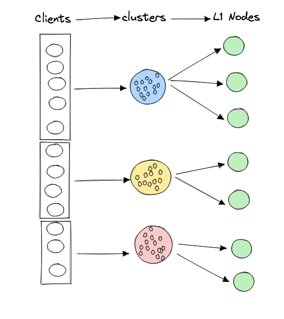
One of the primary challenges in optimizing node selection for a decentralized CDN is the scale of the problem. With around 80 million clients, computing optimal node selections for each individual user becomes computationally intractable. In the classic client-server model, clients are the users accessing the internet, and servers are the Saturn nodes that deliver the requested files to these users. Our job is to match each client with an optimal server (node) to fulfill each request.

The main realization is the following: if you found the optimal node to serve you a file, if your neighbor requests the same file, it is highly likely that that same node is also optimal for them. By doing that we divide the computation we have to do by half. Now think of doing that for a whole neighborhood or a small city, we'd reduce the computation by a few orders of magnitude. Of course, we do lose on some optimality, but the loss is arguably negligible. The quality of selection would be good enough, and "good enough" is the gold standard in engineering.

We implemented DBSCAN (Density-Based Spatial Clustering of Applications with Noise), which is a good fit for identifying clusters of varying shapes and densities in spatial data. By applying DBSCAN to client geographical coordinates, we:

• Reduced millions of individual client optimization problems to hundreds of cluster centers
• Created representative points that could be optimized for all clients in that region
• Enabled consistent experiences for geographically proximate users

The implementation was practical and scalable:

• We only needed a statistically significant sample to identify meaningful clusters
• New clients were assigned to existing clusters based on IP geolocation
• A periodic cronjob dynamically adjusted clusters as client patterns changed

When new clients connected between cluster updates, they would geolocate themselves and find their nearest cluster center. You might notice that having the client geolocate means that when the client connects, there is some delay before they can benefit from the CDN. That is a correct and astute observation, and one of the problems that haunted me for a while.

We used Recursive DBSCAN, which extends DBSCAN to handle varying-density clusters through a hierarchical approach. The implementation requires three key parameters:

1. ε (epsilon): Maximum distance between neighboring points
2. MinPts: Minimum points to form a dense region
3. ξ (xi): Density factor for recursive calls

The algorithm works as follows:

1. Run DBSCAN with initial parameters to identify clusters and noise points

   • Define ε-neighborhood: $N_\varepsilon(p) = \{q \in D \mid \text{dist}(p,q) \leq \varepsilon\}$
   • Core points: $\text{CorePoints} = \{p \in D \mid |N_\varepsilon(p)| \geq \text{MinPts}\}$

2. Recursively process each cluster with reduced parameters:

   • New parameters: $\varepsilon_{new} = \varepsilon \cdot \xi$ and $\text{MinPts}_{new} = \text{MinPts} \cdot \xi$
   • Apply DBSCAN to each cluster if it has enough points

3. Merge subclusters and assign noise points to nearest clusters when appropriate

The density-reachability property ensures coherent clusters at each level, with points connected through a chain of neighbors: $q \text{ is density-reachable from } p \iff \exists p_1,...,p_n: p_1 = p, p_n = q: p_{i+1} \in N_{\varepsilon_k}(p_i) \text{ and } |N_{\varepsilon_k}(p_i)| \geq \text{MinPts}_k$

Selecting Candidate Nodes for Each Cluster

After grouping our clients into geographic clusters using DBSCAN, the next step was to determine which nodes should serve each cluster. We needed a computationally efficient way to select a subset of candidate nodes for each cluster without testing all possible combinations. For example, a node in Australia had no business serving a client in Europe and vice-versa.

Voronoi tessellation is an algorithm that partitions a space into regions based on distance to specific points. Each region contains all points closest to a particular seed point rather than any other seed point, creating natural boundaries of influence.

We implemented a modified Voronoi-based approach that adds a redundancy factor to node selection. For each node in our network, we identified its closest client cluster center and assigned it as a primary candidate server for that cluster. We then also assigned each node to its second-closest cluster center, creating intentional overlap in our node assignments. This redundancy ensures that each cluster has access to lots of nodes and that nodes can serve more than one cluster.

To be concrete, we can define the following:

• $\mathcal{S} = \{s_1, s_2, ..., s_n\}$ as the set of cluster centers
• $\mathcal{N} = \{n_1, n_2, ..., n_m\}$ as the set of nodes in our network
• $d(n_j, s_i)$ as the geographic distance between node $j$ and cluster center $i$

For each node $n_j \in \mathcal{N}$, we compute an ordered set of distances to all cluster centers:

$\mathcal{D}(n_j) = \{d(n_j, s_i) : s_i \in \mathcal{S}\}$

We then define $\pi_{n_j}(k)$ as the index of the $k$-th closest cluster center to node $n_j$:

$\pi_{n_j}(k) = \arg\min_{i \in \{1,2,...,n\} \setminus \{\pi_{n_j}(1), \pi_{n_j}(2), ..., \pi_{n_j}(k-1)\}} d(n_j, s_i)$

For our redundancy factor $r = 2$, we define the assignment function $\mathcal{A}$ such that:

$\mathcal{A}(n_j) = \{s_{\pi_{n_j}(1)}, s_{\pi_{n_j}(2)}\}$

This yields the set of candidate nodes $\mathcal{C}(s_i)$ for each cluster center $s_i$:

$\mathcal{C}(s_i) = \{n_j \in \mathcal{N} : s_i \in \mathcal{A}(n_j)\}$

This approach creates a simple two-tier mapping:

1. Clients → Clusters (based on client location)
2. Clusters → Candidate Nodes (based on Voronoi assignment)

By focusing only on the subset of nodes in a cluster's Voronoi cell, we drastically reduced the computation required for node selection while still achieving optimal performance.

Data Collection

One of the backbones of Saturn was our data collection process. It's not something we built purely for optimizing node selection, but a crucial part of the process since this data would fuel our optimization algorithms.

We implemented a system where clients themselves perform the testing of nodes and report back the results. Each client within a cluster contributed to testing both active nodes (currently serving requests) and candidate nodes (potential future servers). Here's how the process worked:

1. Initial node assignment: When a client connected to the network, it was assigned to a geographic cluster based on its IP location.

2. Node pool distribution: The client received two sets of nodes:

   • Active pool: Nodes currently designated as optimal for their cluster
   • Testing pool: Additional nodes that could potentially serve the cluster in the future

3. Request mirroring: As the client made normal requests to active nodes, it occasionally "mirrored" these requests to nodes in the testing pool at a configurable rate. There was an upper bound to request mirroring to avoid congestion.

4. Performance metrics collection: For each request (both primary and mirrored), clients measured and reported key metrics such as TTFB (time to first byte), total transfer time, any errors, and so on.

5. Telemetry reporting: Clients periodically sent this performance data to our orchestration service, which aggregated it by cluster and node.

Our data collection did rely on self-reporting by clients and nodes on the network. This opened the door for a lot of malicious behavior. We did have fraud detection and put substantial checks in place to counter that. The details of that warrant a separate post, but worth mentioning as fraud would turn out to be a critical problem to solve independent of our optimization.

Computing Node Capacity

An essential aspect of our optimization model was accurately determining each node's capacity by determining on average how many requests per second a node could reliably handle before performance degradation. We implemented node health checks that periodically reported key statistics about hardware performance. By monitoring specific components (CPU utilization, memory usage, disk I/O, network bandwidth) under varying request loads, we identified saturation points for each node.

A node's capacity is essentially limited by its first resource (CPU, Memory, Network, etc.) that saturates first. Once we determined the request threshold at which the first component approached 95% utilization, we set the node's capacity slightly below this value to ensure reliable operation.

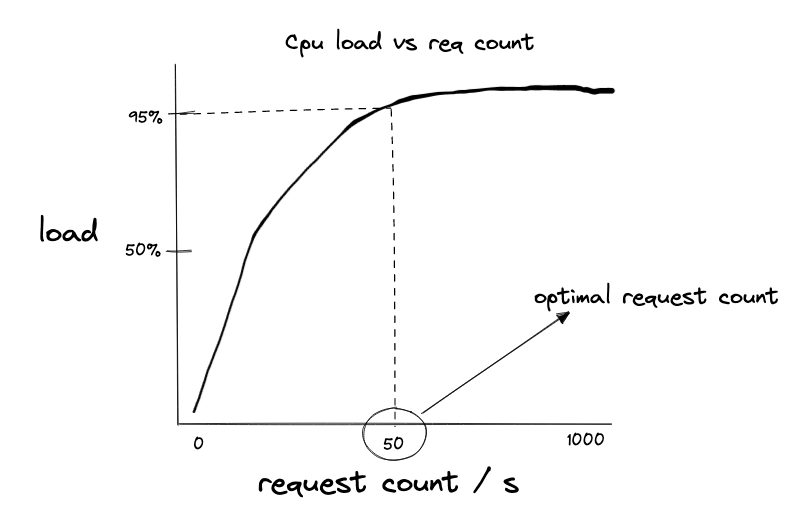
The above graph shows how we determined capacity thresholds for different node types.

With this comprehensive data collection system in place, we were able to extract highly specific performance metrics for each node to drive our node selection optimization:

• Latency percentiles: We calculated p50 (median), p95, and p99 values to understand both typical and worst-case performance scenarios for each node-cluster pair.
• Error rates: The percentage of failed requests.
• Request capacity: Maximum sustainable requests per second before performance degradation
• Download speeds: Average and peak transfer rates for different content sizes
• Availability: Uptime statistics and response consistency over time

Now we Optimize

So far, we've tackled several complex engineering challenges: we grouped millions of clients into manageable geographic clusters, created a system for selecting candidate nodes for each cluster, and built a comprehensive data collection pipeline to measure node performance. Now we arrive at the heart of the system—the algorithm that would actually decide which nodes serve which clusters.

After all that preparatory work, you might expect an equally complex optimization solution. Surprisingly, the answer turned out to be elegantly simple. The actual optimization part was honestly the simplest to solve. The problem setup could be looked at as a constraint optimization problem. Therefore, Linear programming (LP) stood out as a simple and effective technique to resolve this for a few reasons:

1. Well-established solvers: Linear programming has been extensively studied, with highly efficient and reliable solvers available as open-source libraries.
2. Guaranteed optimality: Certain LP algorithms provide globally optimal solutions when the problem can be expressed in terms of bounded linear constraints.
3. Flexibility: We could easily modify our objective function to prioritize different metrics (latency, error rates, throughput) and deploy in seconds. We did that a lot.
4. Scalability: LP problems can be solved quickly even with many variables and constraints.

Our optimization problem for each cluster can be expressed as:

Where:

• $\lambda_i$ represents the proportion of traffic assigned to node $i$
• $f(n_i)$ is our composite performance metric for node $i$. It accounted for things like TTFB, throughput, etc.
• $T$ is the total estimated traffic for the cluster
• $t_i$ is the capacity of node $i$
• $e_i$ is the error rate for node $i$
• $e_{max}$ is our maximum acceptable error rate (set at 0.5%)
• $u_i$ is the uptime for node $i$
• $u_{min}$ is our minimum acceptable uptime (set at 99%)

This optimization can be run on any an open-source LP solver and it can run periodically for each cluster independently. It is also parallelizable for each cluster.

Note that we can also globally optimize for all clusters in one go across all nodes in the network. This would change the equation to minimize to:

$\min_{\lambda} \sum_{i=1}^{n} \sum_{j=1}^{m} \lambda_{ij} \cdot f(n_{ij})$

Where $\lambda_{ij}$ represents the proportion of traffic assigned to node $j$ in cluster $i$, and $f(n_{ij})$ is the performance metric for that specific node.

Implementing the Node Selection

The vector $\{\lambda_1, \lambda_2, \cdots, \lambda_m\}$ output by our optimization algorithm serves as a weighting vector for client traffic distribution. When a client joins our network, it's assigned to a specific geographical cluster $C_k$, and receives the corresponding set of nodes $N_k = \{n_1, n_2, \ldots, n_m\}$ along with their weights $\Lambda_k = \{\lambda_1, \lambda_2, \ldots, \lambda_m\}$.

For each request, the client selects a node using weighted random selection, where the probability $P(n_i)$ of selecting node $n_i$ is directly proportional to its weight: $P(n_i) = \lambda_i \quad \text{where} \sum_{i=1}^{m} \lambda_i = 1$

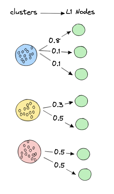
The above visualization shows node weight assignments for a sample cluster. The size of each circle represents the proportion of traffic directed to that node, while the color indicates the node's performance (darker blue = better performance).

The Results & Lessons Learned

These optimization methods saw significant improvements in Saturn's performance metrics compared to our original geographic-based node selection approach:

• ~1.2x improvement in p50 (median) latency (TTFB) from ~51ms to ~44ms across all regions.
• ~1.8x improvement in p95 latency from ~750ms to ~420ms.
• ~2.7x improvement in p99 latency from ~3800ms to ~1400ms.

Working on this CDN was the largest scale and most complex optimization problem I've worked on so far. One of my observations is that the most challenging aspects weren't in the actual optimization algorithm itself but in all the preparatory work: clustering millions of clients effectively, creating meaningful geographic representations, designing a robust data collection system, and defining appropriate constraints and performance metrics. The actual linear programming solver was honestly trivial.

This was also a reminder for myself that in the age of AI/ML hype, traditional optimization techniques still have their place. Many problems can and should be solved by existing mathematical methods rather than defaulting to ML, because they offer a simpler, faster, and interpertable approach that gets the answer right every time.

Overall, this was a lot of fun to work on. Would do it again.